Go Profiling: From pprof to Flame Graphs

Your service is slow. You have a theory — maybe it’s the database query, maybe it’s the JSON serialization, maybe it’s something else entirely. You could guess and change things one by one, deploying each time, hoping the graph gets better. Or you could profile it, look at exactly what your program is actually doing, and know for certain where the time or memory is going.

Profiling is the practice of measuring a running program to find out where it spends resources. Go makes this exceptionally easy compared to most languages — the profiling tools are built into the standard library, the overhead is low enough to run in production, and the tooling is part of the Go CLI itself.

This post is a deep guide. We’ll start from the very beginning — what profiling is, how it works under the hood — and work up through every profile type, how to collect them, how to read them, and how to turn what you see into a fix. If you’re a junior engineer who has never profiled anything before, this is written for you.

---

Why Guessing Doesn’t Scale

Before we get into the tooling, let’s talk about why profiling matters in the first place.

When a program is slow, our instinct is to reason about it. “The database call is probably slow.” “We’re probably doing too much work per request.” These guesses are sometimes right. But they can also lead you down the wrong path — spending days optimizing code that wasn’t actually a bottleneck, while the real problem goes untouched.

The deeper problem is that modern programs are complex. Your request handler calls a logger, which calls a string formatter, which calls an interface method, which calls a reflection-heavy library. Any of those could be the bottleneck. Your intuition, even after years of experience, will miss things that the profiler sees immediately.

There’s a principle in performance work sometimes called Amdahl’s Law: the speedup you get from optimizing a part of the program is limited by how much of the total time that part actually takes. If json.Marshal is 5% of your request time and you make it 10× faster, your overall request time drops by only 4.5%. But if json.Marshal is actually 60% of your request time, the same 10× improvement reduces total request time by 54%. Finding the part that actually dominates is everything.

That’s what profiling gives you — the real numbers, not the guessed ones.

---

How Go Works: Background You Need

To read profiles intelligently, you need a mental model of what Go is doing at runtime. This isn’t deep theory — it’s the concepts you’ll see show up in every profile.

Goroutines and the Scheduler

Go is a concurrent language. Goroutines are lightweight execution threads managed by the Go runtime, not the operating system. You can have thousands or even millions of goroutines in a single process — each uses only a few kilobytes of stack memory (compared to megabytes for an OS thread).

The Go scheduler is called the M:N scheduler because it maps M goroutines onto N OS threads. The scheduler decides which goroutines run, when they run, and on which OS thread. This scheduling happens automatically, and most of the time you don’t need to think about it.

But when you’re profiling, you do need to think about it, because:

• A goroutine that’s “doing work” shows up in a CPU profile
• A goroutine that’s “waiting” (on I/O, a channel, a mutex, a syscall) shows up in a goroutine or block profile
• The scheduler itself can become a bottleneck — this shows up in a trace

The scheduler uses units called P (processor) — you can think of a P as a slot that lets a goroutine actually run. By default, Go sets GOMAXPROCS to the number of logical CPUs on the machine. If you have 8 CPUs, you have 8 Ps, meaning 8 goroutines can run simultaneously.

The Garbage Collector

Go is a garbage-collected language. Memory that you allocate (with make, new, struct literals, slices, maps, interface values, closures, etc.) is managed by the runtime. The GC periodically scans live objects and frees memory that’s no longer reachable.

This is convenient, but it has costs:

1. Allocation itself costs time. Every make([]byte, 1024) is work the runtime has to do.
2. GC cycles cost time. When the GC runs, it uses CPU resources and can pause goroutines.
3. Memory pressure affects GC frequency. If you allocate a lot, the GC runs more often.

The GC uses a stop-the-world (STW) pause to do certain housekeeping tasks. In modern Go (1.14+), these pauses are extremely short — typically under 1 millisecond. But if you’re experiencing latency spikes at the 99th or 99.9th percentile, even a 1ms pause matters. The trace profiler is the tool that surfaces these.

Understanding the GC is critical for reading memory profiles. When you see a function high in the heap profile, it’s because that function is responsible for keeping memory alive — either directly or through a chain of references.

The Stack vs The Heap

In Go, every goroutine has its own stack — a contiguous region of memory where local variables and function call frames live. The stack grows and shrinks automatically. This is fast because allocating on the stack is just a pointer increment.

The heap is shared memory. When the compiler determines that a variable’s lifetime might extend beyond the function that creates it (through escape analysis), it allocates that variable on the heap instead. Heap allocations are slower and create work for the GC.

You don’t control this directly — the compiler decides. But you can influence it, and this is one of the primary levers in memory optimization. When you see “allocations per operation” in a benchmark, it’s measuring how many times the compiler decided to use the heap.

---

How Profiling Actually Works

Before you use a profiler, it helps to understand what it’s doing. Go’s CPU profiler is a sampling profiler.

Here’s the idea: profiling every single instruction a program executes would slow it down enormously and produce too much data to be useful. Instead, a sampling profiler sets up a timer that fires at a regular interval — by default, 100 times per second (every 10 milliseconds). Each time the timer fires, the profiler records the current call stack of every running goroutine. After you collect thousands of these samples, you have a statistical picture of where the program spends its time.

The functions that appear most often in the samples are the ones consuming the most CPU time. Functions that are called rarely or execute quickly appear infrequently.

This means a few important things:

• CPU profiles are statistical, not exact. A function that shows 42.86% of samples took roughly 42.86% of CPU time — it’s an approximation, not a precise measurement.
• Very fast functions may be invisible. If a function completes in under 10ms, it might never be sampled. This is why microbenchmarks (which run functions millions of times) are better for measuring tiny functions.
• The overhead is low because we’re only sampling. At 100 samples/second, the profiler adds roughly 1-5% overhead, which is safe for production.

Memory (heap) profiling works differently — it instruments allocation calls directly, and the runtime samples allocations on average once per 512 KB allocated (probabilistic, not deterministic per-512KB; configurable with runtime.MemProfileRate). Any allocation can trigger a sample; it is not a size filter.

---

The Profile Types — What Each One Tells You

Go provides seven distinct profile types. Each answers a different question about what your program is doing.

CPU Profile

What it measures: Where goroutines spend time when they are actively running — executing code, not waiting.

How to think about it: If you imagine all the time your program spends on the CPU sliced into 10ms intervals, the CPU profile shows you which function was at the top of the call stack during each of those slices. Functions that appear in many slices are consuming significant CPU.

What it won’t tell you: Time spent waiting. If your request handler takes 500ms but 450ms of that is waiting for a database response, the CPU profile might show only 50ms of actual work spread across various functions. The other 450ms doesn’t appear in the CPU profile because the goroutine was sleeping — not running.

When to use it:

• Service is slow AND CPU usage is high (close to 100% on one or more cores)
• You want to optimize a tight computation
• You suspect inefficient algorithms or too much work per request

Heap Profile

What it measures: Memory currently allocated on the heap — specifically, which functions are responsible for keeping that memory alive at the time you take the snapshot.

Two views:

• -inuse_space: how much memory is live right now (not yet freed by GC)
• -inuse_objects: how many objects are live right now
• -alloc_space: total bytes allocated since the program started (even if later freed)
• -alloc_objects: total number of allocations since the program started

How to think about it: -inuse_space tells you what’s holding memory right now — useful for debugging high memory usage. -alloc_space tells you what’s been allocating over time — useful for finding GC pressure even when total memory isn’t that high.

When to use it:

• Service is using more memory than expected
• Memory grows over time and doesn’t come down (potential leak)
• GC is running frequently and you want to reduce allocations

Allocs Profile

The Allocs profile is similar to the Heap profile but defaults to showing allocation counts rather than sizes. It records where allocations happened regardless of whether they’re still live. This is the right profile when you’re investigating GC pressure — you want to know what’s causing frequent GC cycles, not just what’s using memory right now.

Goroutine Profile

What it measures: A snapshot of every goroutine that currently exists, and exactly where each one is paused — its full call stack.

How to think about it: Imagine freezing your program at an instant in time and inspecting every thread of execution. You can see which goroutines are doing useful work, which are waiting on I/O, which are blocked on a channel, and which are stuck waiting for a lock.

When to use it:

• Goroutine count is unexpectedly high and growing (goroutine leak)
• Suspected deadlock — the goroutine dump will show them all waiting on each other
• Requests seem to hang — you can see exactly where the goroutines handling those requests are blocked

Mutex Profile

What it measures: Where goroutines are spending time waiting to acquire a mutex (lock). This is distinct from the goroutine profile because it focuses specifically on contention time — the cumulative time goroutines spent blocked on sync.Mutex or sync.RWMutex.

How to think about it: Multiple goroutines competing for the same lock is serialization — it forces concurrency into a single-threaded bottleneck. The mutex profile shows you which locks are the most contested.

Requires opt-in: Must call runtime.SetMutexProfileFraction(n) to enable. Off by default.

When to use it:

• Service does not scale when you add more CPUs
• CPU usage looks low but throughput isn’t improving with more goroutines
• You suspect lock contention under load

Block Profile

What it measures: Where goroutines block on synchronization primitives: channel sends/receives, select, sync.Mutex, sync.RWMutex, sync.WaitGroup, sync.Cond. It records the time goroutines spent waiting.

How to think about it: While the CPU profile shows busy time, the block profile shows waiting time. If your service is slow but CPU is idle, something is blocking goroutines. The block profile shows you what.

The key distinction from Mutex: Block includes all synchronization, not just mutexes. Channel operations, select blocks, and WaitGroup waits all show up here.

These two profiles overlap on mutex contention — the mutex profile measures wait time on contended unlock paths, while the block profile records goroutines blocking on any sync primitive (channels, select, WaitGroup, Cond, and mutexes). Reach for the mutex profile when you suspect lock contention specifically; reach for the block profile when goroutines are blocking somewhere and you don’t yet know where.

Requires opt-in: Must call runtime.SetBlockProfileRate(n) to enable. Off by default.

When to use it:

• Service is slow but CPU is low (goroutines are waiting, not working)
• Suspected slow I/O paths you want to quantify
• Channel-based communication patterns are causing bottlenecks

Trace

What it measures: A complete timeline of everything that happened: every goroutine’s lifecycle (created, started running, blocked, unblocked, destroyed), every GC phase, processor utilization over time, system calls. This is fundamentally different from other profiles — it’s a recording of events rather than a sample.

How to think about it: All other profiles are statistical summaries. The trace is a recording. If CPU profile is like “we measured CPU usage every 10ms and averaged it,” the trace is “here is the exact sequence of everything that happened, with microsecond timestamps.”

Cost: The trace has significantly higher overhead (~10-20% vs 1-5% for pprof) and generates large files. For a 5-second trace on a busy service, you might get a 100MB file.

When to use it:

• Latency spikes that don’t show up in CPU profiles (because the goroutine was sleeping, not running)
• You suspect GC pauses are causing tail latency issues
• Understanding scheduler behavior — why goroutines aren’t getting CPU time
• Diagnosing GOMAXPROCS-related issues

---

Setting Up Profiling in Your Service

There are three main ways to collect profiles. Which one you use depends on what you’re profiling.

Method 1: HTTP Endpoint (Best for Services)

The most common and practical setup. Import net/http/pprof and it registers a set of HTTP handlers automatically under /debug/pprof/. You then collect profiles on-demand from a running service — either locally, in staging, or in production.

package main

import (
    "log"
    "net/http"
    _ "net/http/pprof" // THIS is the key line — side-effect import registers handlers
)

func main() {
    // Option A: single server (simpler, but exposes pprof on your main port)
    mux := http.NewServeMux()
    mux.HandleFunc("/api/users", handleUsers)
    // pprof handlers are already registered on http.DefaultServeMux
    // so if you're using DefaultServeMux, they're already available

    // Option B: separate debug server on a different port (RECOMMENDED)
    // This way profiling never reaches your public-facing load balancer
    go func() {
        // Only bind to localhost — never 0.0.0.0 for the debug server
        log.Println("Debug server listening on localhost:6060")
        if err := http.ListenAndServe("localhost:6060", nil); err != nil {
            log.Printf("debug server error: %v", err)
        }
    }()

    // Your real service
    log.Println("Service listening on :8080")
    log.Fatal(http.ListenAndServe(":8080", mux))
}

Why a separate port? Security. The /debug/pprof/ endpoint exposes information about your running program — goroutine stacks, memory contents (through goroutine dumps). You don’t want this accessible from the internet. By binding the debug server to localhost:6060, only someone with SSH access to the machine (or on the same internal network) can reach it.

After this setup, every endpoint is available:

GET /debug/pprof/              → Index page (links to all profiles)
GET /debug/pprof/profile       → CPU profile (default 30s, ?seconds=N to change)
GET /debug/pprof/heap          → Heap snapshot
GET /debug/pprof/allocs        → Allocs profile
GET /debug/pprof/goroutine     → Goroutine dump
GET /debug/pprof/mutex         → Mutex contention profile
GET /debug/pprof/block         → Block profile
GET /debug/pprof/trace         → Execution trace (?seconds=N)
GET /debug/pprof/threadcreate  → Thread creation profile
GET /debug/pprof/cmdline       → Command line of the process
GET /debug/pprof/symbol        → Look up symbol names by address

Collecting a CPU profile from a live service:

# This collects 30 seconds of CPU data and opens an interactive session
go tool pprof http://localhost:6060/debug/pprof/profile?seconds=30

# Or download first, analyze later (useful for remote servers)
curl -o cpu.out "http://localhost:6060/debug/pprof/profile?seconds=30"
go tool pprof cpu.out

Collecting a heap profile:

# Snapshot right now
curl -o heap.out "http://localhost:6060/debug/pprof/heap"
go tool pprof -inuse_space heap.out

Method 2: Using the Framework Integration (If You Use One)

If your service uses a web framework, there are usually packages to wire pprof in cleanly:

// With gorilla/mux:
import "github.com/gorilla/mux"
import "net/http/pprof"

func registerDebugRoutes(r *mux.Router) {
    r.PathPrefix("/debug/pprof/").HandlerFunc(pprof.Index)
    r.HandleFunc("/debug/pprof/cmdline", pprof.Cmdline)
    r.HandleFunc("/debug/pprof/profile", pprof.Profile)
    r.HandleFunc("/debug/pprof/symbol", pprof.Symbol)
    r.HandleFunc("/debug/pprof/trace", pprof.Trace)
}

Method 3: Programmatic Profiling (For CLIs and Tests)

For programs that don’t have an HTTP server, or when you want to profile a specific code path directly:

package main

import (
    "os"
    "runtime"
    "runtime/pprof"
)

func main() {
    // --- Start CPU profiling ---
    cpuFile, err := os.Create("cpu.out")
    if err != nil {
        panic(err)
    }
    defer cpuFile.Close()

    if err := pprof.StartCPUProfile(cpuFile); err != nil {
        panic(err)
    }
    defer pprof.StopCPUProfile() // IMPORTANT: must call this before program exits

    // --- Do your work here ---
    doExpensiveWork()

    // --- Take a heap snapshot ---
    // Force a GC first so the snapshot reflects only actually-live objects,
    // not objects that have been allocated but not yet collected
    runtime.GC()

    memFile, err := os.Create("mem.out")
    if err != nil {
        panic(err)
    }
    defer memFile.Close()

    if err := pprof.WriteHeapProfile(memFile); err != nil {
        panic(err)
    }
}

The defer pprof.StopCPUProfile() is critical. If your program calls os.Exit or panics without recover, deferred calls don’t run and the profile file will be incomplete. Normal main returns are fine.

Method 4: Benchmark Profiles

For tight loops or functions you’re actively optimizing, benchmark profiling is the most precise approach:

// user_test.go
package user

import (
    "encoding/json"
    "testing"
)

type User struct {
    ID       int    `json:"id"`
    Name     string `json:"name"`
    Email    string `json:"email"`
    Bio      string `json:"bio"`
}

func BenchmarkMarshalUser(b *testing.B) {
    u := User{
        ID:    42,
        Name:  "Abhimanyu Nagurkar",
        Email: "a@example.com",
        Bio:   "Software engineer, builder, dad.",
    }

    b.ReportAllocs() // Show allocations per operation in the benchmark output
    b.ResetTimer()   // Don't count setup time in the benchmark

    for i := 0; i < b.N; i++ {
        _, err := json.Marshal(u)
        if err != nil {
            b.Fatal(err)
        }
    }
    // In Go 1.24+, prefer `for b.Loop()` — equivalent and clearer.
}

Run and collect:

# Run benchmark and collect both CPU and memory profiles
go test -bench=BenchmarkMarshalUser \
        -benchmem \
        -cpuprofile=cpu.out \
        -memprofile=mem.out \
        -count=3 \
        ./...

# The -benchmem flag makes b.ReportAllocs() output visible even without pprof
# Output:
# BenchmarkMarshalUser-8   1000000   1087 ns/op   232 B/op   4 allocs/op
#                          ^          ^             ^           ^
#                          iterations  time/op      bytes       allocs

The allocs/op number is the key signal for memory optimization. 4 allocations per marshal operation means every single marshal call touches the GC 4 times. If you’re marshaling thousands of responses per second, that’s millions of allocations per second creating GC pressure.

Enabling Mutex and Block Profiling

These two are opt-in because they have measurable overhead. Add this somewhere early in your program:

package main

import (
    "net/http"
    _ "net/http/pprof"
    "runtime"
)

func main() {
    // Mutex profiling: record 1 in every N mutex contention events
    // Lower N = more data but more overhead
    // 0 = disabled (default)
    // 1 = record every single contention (use only in dev/staging)
    // 5 = record 20% of contentions (reasonable for staging)
    runtime.SetMutexProfileFraction(5)

    // Block profiling: SetBlockProfileRate(rate) controls sampling.
    // The runtime samples a blocking event with probability duration / rate —
    // so passing 1 records every event, passing 1_000_000 (1 ms) makes events
    // shorter than 1 ms increasingly rare in the profile.
    // Larger values mean less overhead but coarser data.
    // 0 = disabled (default)
    // 1 = record every single blocking event (high overhead — dev only)
    // 1000 = sample at 1us granularity (reasonable for staging)
    // 1000000 = sample at 1ms granularity (safe for production)
    runtime.SetBlockProfileRate(1000000)

    go func() {
        http.ListenAndServe("localhost:6060", nil)
    }()
    // ... rest of your server
}

Production safety guidance:

• Mutex fraction of 5 (20% sampling) is generally safe in production — you’ll miss some contentions but you’ll find the hot ones.
• Block rate of 1000000 (1 ms granularity) is safe in production. SetBlockProfileRate(rate) controls sampling: the runtime samples a blocking event with probability duration / rate — so passing 1 records every event, passing 1_000_000 (1 ms) makes events shorter than 1 ms increasingly rare in the profile. Larger values mean less overhead but coarser data.
• Heap profiling is always on — no opt-in needed, though you can control the sampling rate with runtime.MemProfileRate.

Tagging Profiles with Labels

When a service handles multiple kinds of work, an unlabeled CPU profile mixes everything together. runtime/pprof.Do lets you attach labels to a goroutine’s profile samples so you can later filter by them.

import "runtime/pprof"

func handleRequest(ctx context.Context, req *Request) {
    pprof.Do(ctx, pprof.Labels("endpoint", req.Path, "tenant", req.TenantID), func(ctx context.Context) {
        // all CPU samples and most heap allocations under this call
        // get tagged with endpoint=... and tenant=...
        process(ctx, req)
    })
}

In pprof, filter with tags and tagfocus/tagignore:

go tool pprof -tagfocus="endpoint=/api/users" cpu.out

Labels are essential when you want to know “which endpoint is dominating CPU?” instead of just “what function?”.

---

Reading Profiles: The CPU Profile

Let’s walk through reading a CPU profile in full detail. This is the most important skill to develop.

Starting an Interactive Session

go tool pprof http://localhost:6060/debug/pprof/profile?seconds=30

After 30 seconds of collection, you’ll see:

Fetching profile over HTTP from http://localhost:6060/debug/pprof/profile?seconds=30
Saved profile in /home/user/pprof/pprof.samples.cpu.001.pb.gz
File: myservice
Type: cpu
Time: Apr 21 2026 10:30:00 UTC (30s)
Duration: 30s, Total samples = 2.8s (9.33%)
Entering interactive mode (type "help" for commands, "o" for options)
(pprof)

A few things to notice:

• Total samples = 2.8s — out of 30 seconds of wall clock time, the profiler captured 2.8 seconds of actual CPU time across all goroutines. This makes sense if you have, say, 4 goroutines all actively doing work.
• The file is saved locally so you can re-analyze it later without re-collecting.

The top Command

Type top or top10 to see the hottest functions:

(pprof) top10
Showing nodes accounting for 2.41s, 86.07% of 2.8s total
Dropped 45 nodes (cum <= 14ms)
Showing top 10 nodes out of 87
      flat  flat%   sum%        cum   cum%
     1.20s 42.86% 42.86%      1.20s 42.86%  syscall.Syscall
     0.60s 21.43% 64.29%      1.80s 64.29%  runtime.mallocgc
     0.22s  7.86% 72.14%      0.22s  7.86%  encoding/json.Marshal
     0.18s  6.43% 78.57%      0.50s 17.86%  db.(*Rows).Next
     0.12s  4.29% 82.86%      0.12s  4.29%  runtime.gcBgMarkWorker
     0.05s  1.79% 84.64%      1.05s 37.50%  main.(*Handler).ServeHTTP
     0.03s  1.07% 85.71%      0.60s 21.43%  main.fetchUsers
     0.01s  0.36% 86.07%      0.01s  0.36%  sync.(*Mutex).Lock

Let’s dissect every column:

flat and flat%: Time spent executing inside this function itself — not in any function it calls. When flat is high, this function is doing the work directly. syscall.Syscall at 1.20s flat means the program spent 1.20 seconds actually executing the syscall instruction. Note that encoding/json.Marshal at 0.22s flat means Marshal itself (not counting the functions it calls internally) used 0.22s.

sum%: Running total of flat%. After syscall.Syscall (42.86%) and mallocgc (21.43%), we’ve accounted for 64.29% of the total CPU time. This helps you know when you’ve found “enough” — once sum% hits 80-90%, you’ve identified the dominant work.

cum and cum%: Cumulative time — the time spent in this function and all functions it calls. main.(*Handler).ServeHTTP has only 0.05s flat but 1.05s cum. That means ServeHTTP itself barely does any work — it just calls other functions (like fetchUsers, which calls db.(*Rows).Next, etc.) and those sub-functions are where the time is.

The key insight: When you see high cum with low flat, the function is a dispatcher — it calls things, it doesn’t do things. Follow the call tree down to find the function with high flat. That’s your target.

Sorting options:

(pprof) top10 -flat    # sort by flat time (default)
(pprof) top10 -cum     # sort by cumulative time
(pprof) top10 -name    # sort alphabetically

The list Command

Once you’ve identified a suspicious function, list shows you the source code with per-line timing:

(pprof) list fetchUsers
Total: 2.8s
ROUTINE ======================== main.fetchUsers in /home/user/service/handler.go
      30ms      600ms (flat, cum) 21.43% of Total
         .          .     45:func (h *Handler) fetchUsers(ctx context.Context, filter string) ([]User, error) {
         .          .     46:    query := fmt.Sprintf("SELECT id, name, email FROM users WHERE name LIKE '%%%s%%'", filter)
      10ms       10ms     47:    rows, err := h.db.QueryContext(ctx, query)
         .          .     48:    if err != nil {
         .          .     49:        return nil, err
         .          .     50:    }
         .          .     51:    defer rows.Close()
         .          .     52:
         .          .     53:    var users []User
      10ms      550ms     54:    for rows.Next() {
         .          .     55:        var u User
      10ms       10ms     56:        if err := rows.Scan(&u.ID, &u.Name, &u.Email); err != nil {
         .          .     57:            return nil, err
         .          .     58:        }
         .          .     59:        users = append(users, u)
         .          .     60:    }
         .          .     61:    return users, nil
         .          .     62:}

The dot . means no samples were recorded at that line. Line 54 (rows.Next()) shows 550ms cumulative — the iteration over the result set is where most time goes. This tells you the database round-trips (fetching rows, network I/O) are the bottleneck, not the Go code.

Also notice line 46: fmt.Sprintf to build the SQL query with %%%s%%. This is a format string building a LIKE query. Every call to this function allocates a new string. For a high-traffic endpoint, this is unnecessary. A parameterized query would be faster and also safer (no SQL injection risk).

The web Command — Real CPU Call Graph

(pprof) web

This opens a call graph in your browser. Each box is a function, arrow weight represents time flowing through that call, and box size corresponds to flat time. Below is the actual pprof call graph generated from the benchmark above:

In the graph, the large red/pink boxes are the hot functions. The runtime nodes (scheduler, GC) dominate because the benchmark allocates heavily enough to keep the GC constantly working — itself a signal that allocation rate is too high. The demo.buildReportSlow and encoding/json.Marshal boxes connect into runtime.mallocgc, showing the allocation chain clearly.

The Flame Graph: The Most Useful Visualization

go tool pprof -http=:8090 cpu.out

This opens a web UI with multiple views including the flame graph. The flame graph is often the best way to understand a profile at a glance.

       ┌─────── json.Marshal ──────┐ ┌── strconv.AppendInt ──┐
    ┌─────────────── main.encodeResponse ───────────────────────────────┐
 ┌──────────────────────── main.(*Handler).ServeHTTP ────────────────────────────────┐
 ┌──────────────────────────────── net/http.(*conn).serve ─────────────────────────────────────────────────┐
 ←─────────────────────────────────────────── 2.8s total ─────────────────────────────────────────────────→

Reading a flame graph:

The X-axis represents total time. The Y-axis represents call stack depth. The bottom of the chart is the entry point (root functions like net/http server code or main). As you go up, you go deeper into the call stack.

Width = time. A function that takes up a wide horizontal area is consuming a lot of CPU time. A narrow bar means it’s fast or rarely called.

The flat top is where the work happens. When a function bar has nothing above it — no caller higher in the stack — that’s a leaf function. It’s where the CPU is actually executing instructions. Wide leaf functions are your optimization targets.

Plateaus indicate hot spots. If you see a “plateau” — a wide flat area at a certain height with nothing above it — that’s a function spending CPU time directly. Clicking on it in the interactive view will highlight all call paths that lead to it.

Thin slivers mean fast functions. A very thin vertical bar means a function is either fast or called infrequently. Ignore these.

The color doesn’t mean hot vs cold in pprof’s default flame graph — it’s just used to distinguish different call paths visually. (Some flame graph tools like Brendan Gregg’s flamegraph.pl do use red for hot functions, but pprof uses color categorically.)

---

Reading Profiles: The Heap Profile

Memory profiles require a slightly different mental model from CPU profiles. You’re not asking “where does time go?” — you’re asking “where is memory being held, and who put it there?”

Before diving into the commands, it helps to understand what the heap profile is actually recording.

What the Heap Profile Records

Every time your Go program allocates memory on the heap, the runtime has an opportunity to record that allocation. By default, the runtime samples allocations on average once per 512 KB allocated (probabilistic, not deterministic per-512KB; controlled by runtime.MemProfileRate). Each sample captures the call stack at the point of allocation — so the profile tells you not just how much memory is alive, but which function allocated it and how it was called.

This is important: the heap profile attributes memory to the function that allocated it, not necessarily the function that’s using it. If json.Marshal allocates a []byte that gets passed up the call stack and stored somewhere, the heap profile will show json.Marshal as the allocating function — even though the long-lived reference is held somewhere higher up.

The Four Heap Profile Views

Every heap profile file contains four distinct datasets. You choose which one to view with a flag:

Flag	What it shows	Best used for
-inuse_space	Bytes currently live on the heap	Debugging high RSS / memory usage
-inuse_objects	Count of objects currently live	Finding which types are numerous
-alloc_space	Total bytes allocated since program start	Debugging GC pressure, high allocation rate
-alloc_objects	Total allocation count since program start	Finding frequently-allocated types

curl -o heap.out "http://localhost:6060/debug/pprof/heap"

go tool pprof -inuse_space   heap.out   # default view
go tool pprof -inuse_objects heap.out
go tool pprof -alloc_space   heap.out
go tool pprof -alloc_objects heap.out

Understanding inuse_space vs alloc_space

This distinction trips up nearly everyone the first time. Let’s be very concrete with a story.

Imagine your HTTP service has been running for 1 hour. During that hour, it processed 100,000 requests. Each request allocated a []byte response buffer of about 50KB, used it, and the GC later freed it. It also built a cache that now holds 200MB of user data.

• alloc_space would show the response buffer allocations prominently: 100,000 × 50KB = ~5GB total allocated over the hour. The cache allocations would also appear here.
• inuse_space would show mainly the cache: the response buffers are all gone (freed), so only the 200MB of live cache data appears.

alloc_space (total ever allocated):
   5.00GB   main.buildResponseBuffer   <-- huge, but all freed
   0.20GB   main.(*UserCache).populate

inuse_space (alive right now):
   0.20GB   main.(*UserCache).populate <-- this is what's in memory
   0.00GB   main.buildResponseBuffer   <-- gone, GC freed it

Rule of thumb:

• High RSS / OOM / kubectl top shows too much memory → use -inuse_space
• High CPU from GC / many GC cycles per second / slow allocation-heavy path → use -alloc_space

Both tell you something real. Sometimes you need both to get the full picture.

Collecting and Opening

# Take a snapshot of the heap right now
curl -o heap.out "http://localhost:6060/debug/pprof/heap"

# Open interactively
go tool pprof -inuse_space heap.out

# Or open the web UI with flame graph
go tool pprof -http=:8090 -inuse_space heap.out

To force a GC before snapshotting heap, call runtime.GC() from inside the process (or via a small admin endpoint you add yourself) — there is no built-in pprof endpoint that triggers GC. In your Go code:

import (
    "runtime"
    "runtime/pprof"
)

// Force GC so the snapshot reflects only truly-live objects
runtime.GC()

f, _ := os.Create("heap.out")
defer f.Close()
pprof.WriteHeapProfile(f)

Real Profile Output: What You’ll Actually See

The outputs below are real — generated by running a benchmark with intentional allocation hot spots using go test -bench=BenchmarkAll -benchmem -cpuprofile=cpu.out -memprofile=mem.out.

The benchmark exercises three patterns:

1. buildReportSlow: builds a string with += in a loop — O(n²) allocations
2. marshalSlow: calls json.Marshal which allocates a full []byte on each call
3. processUsers: calls fmt.Sprintf per user to build labels

Benchmark results — this is what you see before even opening pprof:

BenchmarkBuildReportSlow-11    40176    89214 ns/op    844161 B/op     800 allocs/op
BenchmarkBuildReportFast-11   187976    19255 ns/op     20008 B/op     402 allocs/op
BenchmarkMarshalSlow-11       161523    22209 ns/op     18496 B/op       2 allocs/op
BenchmarkMarshalFast-11       153967    23324 ns/op     41026 B/op       4 allocs/op
BenchmarkProcessUsers-11       69067    52088 ns/op     30093 B/op    1746 allocs/op
BenchmarkAll-11                22957   157441 ns/op    914053 B/op    1407 allocs/op

BenchmarkBuildReportSlow at 800 allocs/op and 844KB per call vs BenchmarkBuildReportFast at 402 allocs/op and 20KB per call — the strings.Builder version uses 42× less memory per call. The -benchmem flag gives you this for free, before you even open pprof.

Reading the top Output for Heap

Running go tool pprof -alloc_space mem.out then top10 -cum on the real profile above:

Type: alloc_space
Duration: 8.11s, Total samples = 36577.85MB

      flat  flat%   sum%        cum   cum%
         0     0%     0%  36574.14MB   100%  demo.BenchmarkAll
         0     0%     0%  36574.14MB   100%  testing.(*B).runN
         0     0%     0%  36573.14MB   100%  testing.(*B).launch
32935.27MB 90.04% 90.04%  33339.32MB 91.15%  demo.buildReportSlow
    0.50MB  0.00% 90.04%   2782.90MB  7.61%  demo.marshalSlow (inline)
 1558.32MB  4.26% 94.30%   2782.40MB  7.61%  encoding/json.Marshal
    0.00MB  0.00% 94.30%   1191.54MB  3.26%  encoding/json.(*encodeState).marshal
    0.00MB  0.00% 94.30%   1191.54MB  3.26%  encoding/json.arrayEncoder.encode
    0.00MB  0.00% 94.30%   1191.54MB  3.26%  encoding/json.sliceEncoder.encode
  266.42MB  0.73% 95.03%    451.92MB  1.24%  demo.processUsers

The flat and cum columns work the same as in CPU profiles, but measure memory instead of time:

• demo.buildReportSlow has 32,935MB flat — it directly allocated nearly 33GB worth of string data over the benchmark run. This is the string concatenation += in a loop, each iteration copying the entire accumulated string into a new allocation.
• demo.marshalSlow has only 0.50MB flat but 2,782MB cum — marshalSlow itself allocates almost nothing, but it calls json.Marshal which allocates the full response []byte on every call. The 0.50MB flat is just the slice header.
• encoding/json.Marshal at 1,558MB flat — these are the actual []byte response buffers being allocated fresh each time.
• demo.processUsers at 266MB flat — all those fmt.Sprintf calls building label strings.

The pattern to read: high flat = this is the allocation site. High cum, low flat = this function is a caller that owns the cost indirectly.

Sorting and filtering:

(pprof) top10 -cum         # show by cumulative (understand call chain ownership)
(pprof) top10 -flat        # show by direct allocation (find the actual allocating line)
(pprof) top -cum -n 20     # top 20 by cum

Start with -cum to find which part of the call tree is responsible, then switch to -flat to find the exact function doing the allocating.

Drilling Into Source with list

Once top points you at a function, list shows the exact lines:

(pprof) list buildReportSlow
Total: 36577.85MB
ROUTINE ======================== demo.buildReportSlow
   32.16GB    32.56GB (flat, cum) 91.15% of Total
         .          .     23:func buildReportSlow(users []User) string {
         .          .     24:    result := ""
         .          .     25:    for _, u := range users {
         .          .     26:        // Each + allocates a new string
   32.16GB    32.56GB     27:        result += fmt.Sprintf("User %d: %s <%s>\n", u.ID, u.Name, u.Email)
         .          .     28:    }
         .          .     29:    return result
         .          .     30:}

Line 27 is the entire problem — 32GB attributed to one line (this is total bytes allocated and freed across all benchmark iterations, not memory live at any one moment). Every += on a string in Go creates a brand new string by copying the old string plus the new suffix. With 200 users, that’s 200 copies of increasing length: copy 0 chars, copy ~40 chars, copy ~80 chars, … copy ~8000 chars. Total work is O(n²) in the length of the result.

The tree output confirms the call chain:

(pprof) tree buildReportSlow
----------------------------------------------------------+-------------
      flat  flat%   sum%        cum  cum%   calls calls% + context
----------------------------------------------------------+-------------
                               33339.32MB 100% |   demo.BenchmarkAll
32935.27MB 90.04% 90.04%  33339.32MB 91.15%   |   demo.buildReportSlow
                                 404.06MB  1.21% |     fmt.Sprintf
----------------------------------------------------------+-------------
                                 404.06MB 100% |   demo.buildReportSlow
  368.02MB  1.01% 91.05%    404.06MB  1.10%   |   fmt.Sprintf
----------------------------------------------------------+-------------

buildReportSlow owns 90% of all allocations. fmt.Sprintf inside it accounts for another 404MB (the intermediate formatted strings). The string concatenation itself — the += — is the 32GB, because every loop iteration copies all previous output.

Real Memory Call Graph

Here is the actual go tool pprof -alloc_space -svg mem.out output from the same benchmark — a real memory call graph, not a diagram:

demo.buildReportSlow dominates the graph at 90% of total allocations — its box is the largest. The arrows flow down into fmt.Sprintf and runtime.mallocgc. encoding/json.Marshal is the second cluster. The relative box sizes make the 90/8/2 split visible at a glance.

To generate this yourself from any profile:

go tool pprof -alloc_space -svg mem.out > mem-callgraph.svg
go tool pprof -svg cpu.out > cpu-callgraph.svg

Requires Graphviz (brew install graphviz on macOS).

Using the Heap Flame Graph

The interactive flame graph is the fastest way to see the allocation picture at a glance. Run:

go tool pprof -http=:8090 -alloc_space mem.out

Your browser opens at localhost:8090. Click Flame Graph in the top nav. For the profile above, you’d see a single dominant bar — buildReportSlow taking up ~90% of the horizontal width, with marshalSlow/json.Marshal occupying the remaining ~8%. The overwhelming width of buildReportSlow makes the problem impossible to miss visually; you don’t even need to read the numbers.

Here’s the real pprof flame graph captured from running this exact benchmark:

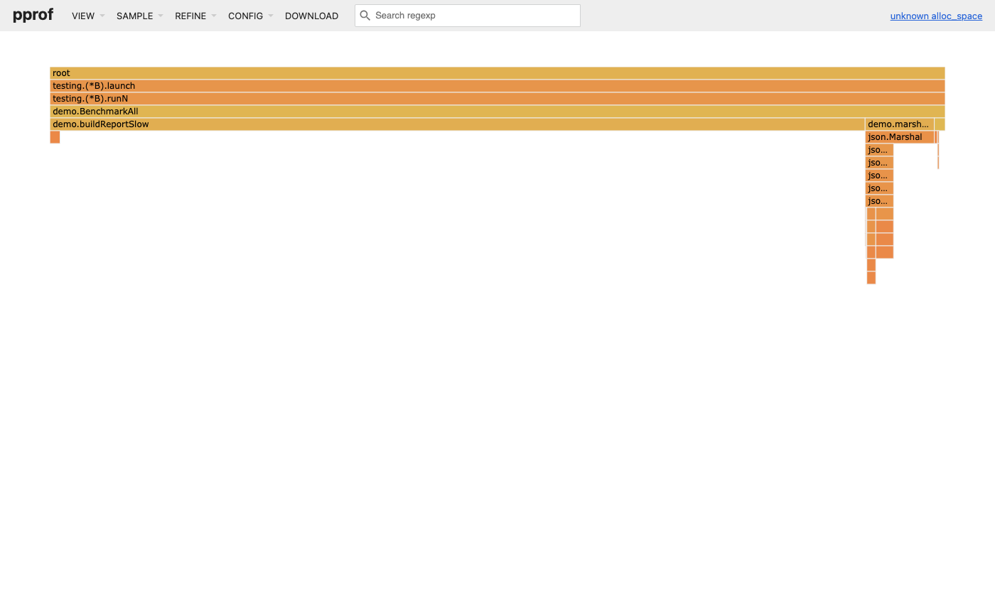
In the web UI, the flame graph for heap profiles reads exactly like the CPU flame graph, but width = memory. A wide bar means that call path is responsible for a lot of allocated memory.

Switch between views in the top navigation:

• Flame graph: visual call tree
• Top: the top table
• Source: annotated source (same as list)
• Peek: shows callers of a function

One particularly useful feature: in the flame graph, you can click a function bar to filter the view to only that function’s subtree. This helps when a big allocator like json.Marshal appears in many call paths — you can isolate just the path you care about.

The -base Flag: Finding What Grew

The most powerful technique for tracking memory leaks is taking two snapshots and comparing them. The diff tells you exactly what grew — not what’s large in general, but what’s larger now than before.

# Step 1: take the first snapshot before the suspected leak period
curl -o heap1.out "http://localhost:6060/debug/pprof/heap"
echo "Snapshot 1 at $(date)"

# Step 2: let the service run for a while under normal traffic
# The leak will accumulate during this time

# Step 3: take the second snapshot
curl -o heap2.out "http://localhost:6060/debug/pprof/heap"
echo "Snapshot 2 at $(date)"

# Step 4: diff them — what grew?
go tool pprof -inuse_space -base heap1.out heap2.out

The output now shows deltas — positive numbers mean that function is holding more memory in snapshot 2:

(pprof) top10
Showing nodes accounting for +52.40MB
      flat  flat%   sum%        cum   cum%
  +42.00MB 80.15% 80.15%  +42.00MB 80.15%  main.(*EventStore).Append
  +10.40MB 19.85% 100.00%  +52.40MB 100.00%  main.(*MetricsCollector).Record

If you see a function with steadily growing positive values across multiple snapshots taken over time, that’s your leak.

Taking periodic snapshots automatically:

For production leak investigations, a simple shell loop works well:

for i in 1 2 3 4 5; do
    curl -s -o "heap_$i.out" "http://prod-host:6060/debug/pprof/heap"
    echo "Snapshot $i at $(date)"
    sleep 300  # 5 minutes between snapshots
done

# Then compare snapshot 1 vs 5 to see total growth
go tool pprof -inuse_space -base heap_1.out heap_5.out

# And compare consecutive snapshots to see the rate of growth
go tool pprof -inuse_space -base heap_1.out heap_2.out
go tool pprof -inuse_space -base heap_2.out heap_3.out

If the growth is consistent across consecutive diffs, the leak is active throughout. If only some diffs show growth, the leak might be triggered by a specific condition (a particular request type, time-of-day behavior, etc.).

Understanding Memory Profile Sampling

Heap profiling is not 100% complete — it’s sampled. By default, the runtime samples allocations on average once per 512 KB allocated (probabilistic, not deterministic per-512KB). This means small allocations that happen infrequently might not appear in the profile.

You can lower the sampling threshold to catch smaller allocations:

import "runtime"

func init() {
    // Record every single allocation (maximum detail, higher overhead)
    // Default is 512*1024 (512KB)
    runtime.MemProfileRate = 1
}

Setting MemProfileRate = 1 means every allocation is recorded. This is useful when investigating a suspected small-object leak that isn’t showing up in the default profile, but it increases overhead significantly and should only be used for targeted debugging, not in production.

What “RSS vs Heap” Means and Why They Differ

One thing that confuses people: the heap profile might show 200MB live but your process’s RSS (resident set size — what top or kubectl top reports) might be 400MB. Why the gap?

Several reasons:

1. Go runtime overhead: The Go scheduler, goroutine stacks, internal runtime structures, and metadata all consume memory that doesn’t show up in the heap profile.
2. Stack memory: Each goroutine has a stack. 1,000 goroutines × 8KB minimum stack = 8MB just in stacks. Stacks can grow much larger.
3. Memory fragmentation: The OS allocates memory in pages (typically 4KB or larger). Even if your heap objects total 200MB, the OS might have mapped 250MB of pages to the process.
4. Go’s memory retention: Go doesn’t immediately return freed memory to the OS. After the GC frees objects, the memory stays in Go’s heap arena until the OS explicitly needs it back or until runtime.FreeOSMemory() is called (or MADV_FREE/MADV_DONTNEED is used on Linux).

If you need to shrink RSS without reducing actual live memory, you can call debug.FreeOSMemory(), which forces the runtime to return unused heap pages to the OS. This is a one-shot operation though — it doesn’t change the long-term allocation pattern.

import "runtime/debug"

// Force return of unused memory pages to the OS
// Rarely needed — the runtime handles this automatically over time
debug.FreeOSMemory()

Using runtime/metrics for Continuous Monitoring

Instead of taking snapshots manually, you can expose heap metrics continuously via runtime/metrics (Go 1.16+):

package main

import (
    "fmt"
    "runtime/metrics"
)

func printHeapStats() {
    // Define which metrics you want
    samples := []metrics.Sample{
        {Name: "/memory/classes/heap/objects:bytes"},   // live heap objects
        {Name: "/memory/classes/heap/released:bytes"},  // released to OS
        {Name: "/memory/classes/heap/free:bytes"},      // free but retained
        {Name: "/gc/heap/allocs:bytes"},                 // cumulative allocs
        {Name: "/gc/cycles/total:gc-cycles"},            // total GC cycles
    }

    metrics.Read(samples)

    for _, s := range samples {
        if s.Value.Kind() == metrics.KindUint64 {
            fmt.Printf("%s = %d\n", s.Name, s.Value.Uint64())
        }
    }
}

Exposing these as Prometheus or Datadog metrics gives you continuous visibility without needing to collect pprof snapshots. You’d typically alert on heap/objects:bytes growing without bound over days, and then use pprof snapshots to investigate the cause once the alert fires.

---

Reading Profiles: Goroutine Dumps

The goroutine profile is different from CPU and heap — it’s not a statistical sample. It’s an instant snapshot of every goroutine that exists right now, with their complete call stacks.

Collecting

# debug=1: just goroutine counts per state
curl "http://localhost:6060/debug/pprof/goroutine?debug=1"

# debug=2: full stack traces for every goroutine (this is what you want)
curl "http://localhost:6060/debug/pprof/goroutine?debug=2"

What a Goroutine Dump Looks Like

goroutine 1 [running]:
main.main()
    /home/user/service/main.go:42 +0x1a4

goroutine 18 [sleep]:
time.Sleep(0x77359400)
    /usr/local/go/src/runtime/time.go:195 +0xd2
main.backgroundJob()
    /home/user/service/jobs.go:23 +0x45
created by main.startJobs in goroutine 1
    /home/user/service/main.go:38 +0x6e

goroutine 23 [chan receive]:
main.processQueue(0xc00012a000)
    /home/user/service/worker.go:45 +0x89
created by main.startWorkers in goroutine 1
    /home/user/service/main.go:52 +0xb2

goroutine 24 [chan receive]:
main.processQueue(0xc00012a000)
    /home/user/service/worker.go:45 +0x89
created by main.startWorkers in goroutine 1
    /home/user/service/main.go:52 +0xb2

... (200 more goroutines in exactly the same state)

The goroutine state is the critical signal. Each goroutine shows its current state in brackets:

• [running] — currently executing on a CPU
• [sleep] — in time.Sleep() or similar
• [chan receive] — blocked waiting for a channel to have data
• [chan send] — blocked waiting for a channel to accept data
• [IO wait] — blocked on I/O (network, file)
• [semacquire] — waiting to acquire a mutex or semaphore
• [select] — blocked in a select statement
• [syscall] — executing a system call

What to look for:

1. Goroutine count that’s unexpectedly high. A healthy service might have hundreds of goroutines — one per active HTTP connection, some for background jobs, some for the runtime itself. But if you see 10,000 goroutines and you have only 100 active requests, something is leaking.

2. Many goroutines in the same state at the same call stack. If you see 500 goroutines all sitting at chan receive on the exact same line, that’s a single channel nobody is reading from. Everything that tries to write to it blocks.

3. Goroutines stuck in syscall state for a long time. System calls should be brief. A goroutine that’s been in syscall for a long time (seconds) is likely doing a blocking network operation with no timeout.

4. created by X pointing to the same place. If you see thousands of goroutines all created by the same function, that function is creating goroutines faster than they’re completing.

Goroutine Leak Example

Here’s a classic goroutine leak pattern and what it looks like in a dump:

// BUGGY CODE: this leaks a goroutine every time processRequest is called
func processRequest(req *Request) {
    resultCh := make(chan Result)  // unbuffered channel

    go func() {
        result := doExpensiveWork(req)
        resultCh <- result  // THIS BLOCKS if nobody reads the channel
    }()

    select {
    case result := <-resultCh:
        sendResponse(result)
    case <-time.After(100 * time.Millisecond):
        sendTimeout()
        // We return here but the goroutine is still running, blocked on resultCh <- result
        // Nobody will ever read from resultCh now
        // The goroutine is leaked
        return
    }
}

In the goroutine dump, you’d see hundreds of goroutines like:

goroutine 1842 [chan send, 45 minutes]:
main.processRequest.func1()
    /home/user/service/handler.go:67 +0x94
created by main.processRequest in goroutine 1234
    /home/user/service/handler.go:62 +0x4e

The 45 minutes shows how long the goroutine has been blocked — a clear sign it’s stuck forever.

The fix:

func processRequest(req *Request) {
    // Use a context with timeout so the goroutine gets a signal to stop
    ctx, cancel := context.WithTimeout(context.Background(), 100*time.Millisecond)
    defer cancel() // This signals the goroutine even if we return early

    resultCh := make(chan Result, 1) // Buffered — goroutine can always send

    go func() {
        result := doExpensiveWork(ctx, req) // Pass ctx so work can abort
        select {
        case resultCh <- result:
        case <-ctx.Done(): // If timeout happened, don't block
        }
    }()

    select {
    case result := <-resultCh:
        sendResponse(result)
    case <-ctx.Done():
        sendTimeout()
    }
}

---

Reading Profiles: The Execution Trace

The trace is the most powerful profiling tool but also the most complex to interpret. Use it when other profiles haven’t given you the answer.

Collecting and Opening

# Collect 5 seconds of trace (use a short window — files get large fast)
curl -o trace.out "http://localhost:6060/debug/pprof/trace?seconds=5"

# Open in browser
go tool trace trace.out

This opens a browser UI at http://localhost:PORT/ with several views.

The Views and What They Tell You

Goroutine analysis — This shows time breakdown per goroutine across five states:

• Execution time: goroutine was running on a CPU
• Network wait: goroutine was waiting for network I/O
• Sync block: goroutine was waiting on a mutex/channel/semaphore
• Scheduler wait: goroutine was ready to run but waiting for a CPU slot
• GC time: goroutine was paused or helping with GC

A goroutine with 10% Execution and 80% Sync block is spending most of its time waiting — likely for a slow database or a contested lock.

View trace — The raw timeline view. You see:

• All goroutines as horizontal lanes
• Color indicates state (running, blocked, network wait, etc.)
• GC events shown as spans that overlay the goroutine timeline
• You can zoom in to microsecond resolution

If you see periodic “gaps” across all goroutines at the same time — that’s a GC stop-the-world pause. The length of that gap is your STW pause latency.

Minimum Mutator Utilization (MMU) — This chart directly answers “what percentage of the time was my code actually running (as opposed to being stopped for GC)?” The Y-axis is utilization (1.0 = 100% of time running), the X-axis is window size (looking at any N-second window, what’s the minimum utilization?). If the MMU at 1ms is 0.80, it means in the worst case, your code was only running 80% of the time in any 1ms window — 20% was GC pauses.

---

Mutex and Block Profiles in Detail

Mutex Profile

After enabling with runtime.SetMutexProfileFraction(5):

go tool pprof http://localhost:6060/debug/pprof/mutex

(pprof) top5
Showing nodes accounting for 8.50s, 95.25% of 8.92s total
      flat  flat%   sum%        cum   cum%
     4.20s 47.09% 47.09%      4.20s 47.09%  sync.(*Mutex).Unlock
     2.10s 23.54% 70.63%      6.30s 70.63%  main.(*Cache).Get
     1.50s 16.82% 87.45%      1.50s 16.82%  main.(*Cache).Set

The times here represent how long other goroutines waited because of contention on this mutex. Cache.Get causing 6.3s of contention means goroutines collectively waited 6.3 seconds trying to acquire the cache’s lock.

The fix pattern: if reads far outnumber writes, switch from sync.Mutex to sync.RWMutex and use RLock()/RUnlock() for reads. Multiple goroutines can hold an RLock simultaneously — only writers need exclusive access.

// Before: every operation, read or write, blocks everyone
type Cache struct {
    mu    sync.Mutex
    items map[string]string
}

func (c *Cache) Get(key string) (string, bool) {
    c.mu.Lock()
    defer c.mu.Unlock()
    v, ok := c.items[key]
    return v, ok
}

// After: reads can happen concurrently, only writes are exclusive
type Cache struct {
    mu    sync.RWMutex
    items map[string]string
}

func (c *Cache) Get(key string) (string, bool) {
    c.mu.RLock()         // Multiple goroutines can hold RLock simultaneously
    defer c.mu.RUnlock()
    v, ok := c.items[key]
    return v, ok
}

func (c *Cache) Set(key, value string) {
    c.mu.Lock()          // Only one writer at a time
    defer c.mu.Unlock()
    c.items[key] = value
}

Block Profile

After enabling with runtime.SetBlockProfileRate(1):

go tool pprof http://localhost:6060/debug/pprof/block

(pprof) top5
Showing nodes accounting for 15.2s, 87.36% of 17.4s total
      flat  flat%   sum%        cum   cum%
     8.40s 48.28% 48.28%      8.40s 48.28%  main.(*DB).query
     4.20s 24.14% 72.41%      4.20s 24.14%  runtime.selectgo
     2.10s 12.07% 84.48%      2.10s 12.07%  sync.(*WaitGroup).Wait

DB.query blocking 8.4s means goroutines spent 8.4 seconds waiting in that function. Combined with looking at the source code, this usually means waiting on a connection pool (not enough connections available) or slow query results.

runtime.selectgo blocking means goroutines are blocking in select statements — either waiting for a channel or a timeout. This might be expected (workers waiting for jobs) or a sign of slow producers.

---

Common Scenarios: Step-by-Step Walkthroughs

Scenario 1: The “Everything Is Slow” Investigation

You get a report: “The API is slow.” P50 is 200ms, P99 is 2 seconds. CPU is at 60%. Where do you start?

Step 1: CPU profile first because CPU is elevated.

# Generate some load first (use hey, wrk, or k6)
hey -n 10000 -c 50 http://localhost:8080/api/users

# In another terminal, collect the profile
go tool pprof http://localhost:6060/debug/pprof/profile?seconds=30

(pprof) top10
      flat  flat%   sum%        cum   cum%
     1.80s 64.29% 64.29%      1.80s 64.29%  runtime.mallocgc
     0.40s 14.29% 78.57%      0.40s 14.29%  encoding/json.Marshal
     0.30s 10.71% 89.29%      2.50s 89.29%  main.(*Handler).getUsers

mallocgc is the garbage collector’s allocation function. It being at 64% means the program is spending most of its CPU time allocating memory, not doing actual work. This is GC pressure — the allocation rate is so high that the GC can’t keep up.

Step 2: Find what’s allocating.

# Get the allocs profile (not heap — allocs shows total allocation rate)
go tool pprof http://localhost:6060/debug/pprof/allocs

(pprof) top10 -alloc_space
      flat  flat%   sum%        cum   cum%
  1.20GB 48.00% 48.00%    1.20GB 48.00%  encoding/json.Marshal
  0.80GB 32.00% 80.00%    2.00GB 80.00%  main.(*Handler).getUsers
  0.30GB 12.00% 92.00%    0.30GB 12.00%  fmt.Sprintf

json.Marshal is allocating 1.2GB total (this is over the 30 second period). For 10,000 requests, that’s 120KB of allocation per request just for JSON serialization.

Step 3: List the hot function.

(pprof) list getUsers
...
     .     1.2GB     78:    data, err := json.Marshal(users)

Every request is marshaling a potentially large users slice into JSON from scratch. Fixes:

1. Use json.NewEncoder(w).Encode(users) — streams directly to the response writer, avoids allocating the []byte intermediate
2. If the data is cacheable, cache the serialized result
3. Use sync.Pool for the encoder itself

Step 4: Implement, re-profile, confirm.

// Before
func (h *Handler) getUsers(w http.ResponseWriter, r *http.Request) {
    users, _ := h.store.ListUsers()
    data, err := json.Marshal(users)    // allocates a []byte
    if err != nil {
        http.Error(w, err.Error(), 500)
        return
    }
    w.Header().Set("Content-Type", "application/json")
    w.Write(data)
}

// After
func (h *Handler) getUsers(w http.ResponseWriter, r *http.Request) {
    users, _ := h.store.ListUsers()
    w.Header().Set("Content-Type", "application/json")
    // json.NewEncoder streams to w directly — no intermediate allocation
    if err := json.NewEncoder(w).Encode(users); err != nil {
        // Can't set status code here (headers already sent), so log it
        log.Printf("encode error: %v", err)
    }
}

Re-profile and compare. The mallocgc entry should drop significantly.

Scenario 2: Memory Leak Investigation

You notice your service’s memory usage grows by about 50MB per hour and never comes back down. The service runs fine for a day but needs to be restarted weekly.

Step 1: Capture two snapshots separated by time.

# Capture the first snapshot (note the time)
curl -o heap1.out "http://localhost:6060/debug/pprof/heap"
echo "Snapshot 1 taken at $(date)"

# Wait 1 hour, or until you see significant memory growth
sleep 3600

# Capture the second snapshot
curl -o heap2.out "http://localhost:6060/debug/pprof/heap"
echo "Snapshot 2 taken at $(date)"

Step 2: Compare.

go tool pprof -inuse_space -base heap1.out heap2.out

(pprof) top5
Showing nodes accounting for +52.40MB
      flat  flat%   sum%        cum   cum%
  +42.00MB 80.15% 80.15%  +42.00MB 80.15%  main.(*EventStore).Append
  +10.40MB 19.85% 100.00%  +52.40MB 100.00%  main.(*MetricsCollector).Record

EventStore.Append grew by 42MB. This is your leak.

Step 3: Inspect the code.

// Probable buggy code
type EventStore struct {
    events []Event  // this slice grows unboundedly
    mu     sync.Mutex
}

func (s *EventStore) Append(e Event) {
    s.mu.Lock()
    defer s.mu.Unlock()
    s.events = append(s.events, e)  // never trimmed, never rotated
}

The events slice keeps all events forever with no eviction, rotation, or size limit.

Fix options:

1. Keep only the last N events with a ring buffer
2. Write events to an external store (database, message queue) and don’t keep them in memory
3. Add a TTL-based eviction: periodically trim events older than some duration

Scenario 3: Diagnosing p99 Latency Spikes

P50 is 10ms, P99 is 500ms. The requests that are slow seem random — no pattern in the payload. CPU is low, memory is stable. This is a classic GC pause pattern.

Step 1: Capture a trace during load.

# Apply load
hey -n 5000 -c 100 http://localhost:8080/api/data

# Capture trace simultaneously (5 second window is usually enough)
curl -o trace.out "http://localhost:6060/debug/pprof/trace?seconds=5"
go tool trace trace.out

In the browser, open “View trace” and zoom in on the timeline. Look for moments where all goroutines stop simultaneously. These are GC stop-the-world pauses.

You might see:

STW mark termination: 2.3ms
STW sweep termination: 0.1ms
STW mark termination: 1.8ms
... repeating every 200ms ...

2.3ms STW pauses every 200ms. At 100 concurrent requests, a 2.3ms pause would cause all in-flight requests to stall. For a request that took 8ms without the pause, it now takes 10.3ms. But if a request is unlucky and hits two pauses, it takes 12.6ms. At p99, you’re seeing multiple pauses accumulate.

Step 2: Check allocation rate.

In the trace UI, look at “Goroutine analysis” and look at the GC goroutines. If gcBgMarkWorker is constantly present, the GC is running continuously — a sign of very high allocation rate.

Step 3: Reduce allocation rate.

The most effective fix is using sync.Pool for frequently-allocated objects:

// Before: every request allocates a new buffer
func handleRequest(w http.ResponseWriter, r *http.Request) {
    buf := new(bytes.Buffer)  // new allocation every request
    buildResponse(buf, r)
    w.Write(buf.Bytes())
}

// After: reuse buffers from a pool
var bufPool = sync.Pool{
    New: func() any {
        return new(bytes.Buffer)
    },
}

func handleRequest(w http.ResponseWriter, r *http.Request) {
    buf := bufPool.Get().(*bytes.Buffer)
    buf.Reset()              // clear the buffer before use
    defer bufPool.Put(buf)   // return to pool when done

    buildResponse(buf, r)
    w.Write(buf.Bytes())
}

sync.Pool maintains a pool of objects that can be reused across goroutines. The GC clears the pool on each GC cycle (so pool objects don’t prevent garbage collection), but in the steady state between GC cycles, goroutines reuse the same buffer objects instead of allocating new ones.

Step 4: Tune the GC target if needed.

If you’ve reduced allocations and still see GC pressure, you can tune when the GC triggers:

import "runtime/debug"

func main() {
    // GOGC controls when GC triggers. Default is 100, meaning GC triggers
    // when heap grows 100% beyond the size after the last GC.
    // Setting to 200 means GC triggers less often but uses more memory.
    // This is a trade-off: less GC CPU, more RAM usage.
    debug.SetGCPercent(200)

    // GOMEMLIMIT (Go 1.19+) sets a soft memory limit.
    // The GC will work harder to stay under this limit.
    // This prevents the service from using so much memory it gets OOM-killed.
    debug.SetMemoryLimit(1 << 30) // 1 GB

    // ... rest of your program
}

Or via environment variables (no code change needed):

GOGC=200 GOMEMLIMIT=1073741824 ./myservice

Scenario 4: The Service Doesn’t Scale Under Load

Adding more CPUs (or increasing GOMAXPROCS) doesn’t improve throughput. This suggests serialization — something is forcing work to happen one at a time.

Profile: Mutex contention.

# Make sure SetMutexProfileFraction was called at startup
go tool pprof http://localhost:6060/debug/pprof/mutex

(pprof) top5
      flat  flat%   sum%        cum   cum%
    12.30s 68.33% 68.33%     12.30s 68.33%  main.(*RequestCounter).Increment
     4.20s 23.33% 91.67%      4.20s 23.33%  main.(*RateLimiter).Allow

A RequestCounter that’s being incremented on every request from every goroutine is a global shared state with a mutex. Every goroutine contends on it.

Fix: Use sync/atomic for simple counters.

// Before: mutex-protected counter is a bottleneck
type RequestCounter struct {
    mu    sync.Mutex
    count int64
}

func (c *RequestCounter) Increment() {
    c.mu.Lock()
    c.count++
    c.mu.Unlock()
}

func (c *RequestCounter) Get() int64 {
    c.mu.Lock()
    defer c.mu.Unlock()
    return c.count
}

// After: atomic operations require no lock
type RequestCounter struct {
    count int64 // must be 64-bit aligned for atomic ops (automatic on 64-bit platforms when the field is the first in the struct; matters on 32-bit ARM/x86 if you reorder fields)
}

func (c *RequestCounter) Increment() {
    atomic.AddInt64(&c.count, 1) // lock-free, safe from multiple goroutines
}

func (c *RequestCounter) Get() int64 {
    return atomic.LoadInt64(&c.count)
}

For more complex shared data structures, consider sharding — splitting one lock into N locks by key:

// Instead of one global cache with one lock:
type ShardedCache struct {
    shards [256]struct {
        mu    sync.RWMutex
        items map[string]string
    }
}

func (c *ShardedCache) shard(key string) int {
    // Simple hash to pick a shard
    h := fnv.New32a()
    h.Write([]byte(key))
    return int(h.Sum32()) % 256
}

func (c *ShardedCache) Get(key string) (string, bool) {
    s := c.shard(key)
    c.shards[s].mu.RLock()
    defer c.shards[s].mu.RUnlock()
    v, ok := c.shards[s].items[key]
    return v, ok
}

Now instead of all 256 goroutines contending on a single lock, each goroutine contends with only ~1 other goroutine on average (because keys are distributed across 256 shards).

---

Visual Guide: Reading Flame Graphs and Memory Diagrams

This section walks through what the go tool pprof web UI actually looks like and how to navigate it. Since screenshots from a live pprof session depend on your specific program, the annotated diagrams below replicate the structure and layout of what you’ll see — so when you open the real UI, you’ll know exactly what you’re looking at.

Opening the Web UI

go tool pprof -http=:8090 cpu.out

Your browser opens to http://localhost:8090. The top navigation bar has these views:

[ Top ] [ Graph ] [ Flame Graph ] [ Peek ] [ Source ] [ Disassemble ]
                                      ^
                                  start here

Top — the top table you’ve already seen in the interactive CLI. Good first stop.

Graph — a directed call graph. Boxes are functions, arrows show call relationships, box size corresponds to flat cost, arrow weight corresponds to flow. Gets cluttered on large profiles but good for seeing call relationships.

Flame Graph — the flame graph. Best for understanding the full picture at a glance.

Peek — shows callers of the selected function. Useful for understanding who is responsible for a hot function you didn’t write.

Source — annotated source, same as the list command.

---

Anatomy of a CPU Flame Graph

Here’s what a CPU flame graph looks like for a typical HTTP service, annotated:

 WIDE AND AT THE TOP = hot leaf function (where CPU is burning)
 │
 │    ┌──────────────────────────────────────────────┐
 │    │          encoding/json.(*Encoder).Encode     │  ← 38% CPU, this is hot
 │    └──────────────────────────────────────────────┘
 │    ┌─────────────────────────────────────────────────────────────────┐
 │    │                   main.buildAPIResponse                         │
 │    └─────────────────────────────────────────────────────────────────┘
 │    ┌──────────────────────────────────────────────────────────────────────────────────┐
 │    │                           main.(*Handler).ServeHTTP                              │
 │    └──────────────────────────────────────────────────────────────────────────────────┘
 │    ┌──────────────────────────────────────────────────────────────────────────────────────────┐
 │    │                              net/http.(*conn).serve                                       │
 │    └──────────────────────────────────────────────────────────────────────────────────────────────┘
 ↓
 WIDE AND AT THE BOTTOM = root of the call stack (entry point)

Key patterns to recognize:

Pattern 1 — Flat top (direct hot spot)

 ┌────────────────────────────────────┐
 │         syscall.RawSyscall         │  ← wide, nothing above it
 └────────────────────────────────────┘  ← this IS the bottleneck
 ┌─────────────────────────────────────────┐
 │         net.(*netFD).Read               │
 └─────────────────────────────────────────┘
 ┌──────────────────────────────────────────────────────┐
 │             bufio.(*Reader).fill                     │
 └──────────────────────────────────────────────────────┘

syscall.RawSyscall has no children (nothing above it). The CPU is spending time executing the system call directly. The fix is either to reduce the number of syscalls (buffering, batching) or accept that I/O is the bound.

Pattern 2 — Wide middle (delegating hot spot)

                         ┌──────┐ ┌──────┐
                         │ fmt  │ │strco │  ← many small children
                         └──────┘ └──────┘
 ┌─────────────────────────────────────────────────────────────┐
 │                  encoding/json.Marshal                       │  ← wide, has children
 └─────────────────────────────────────────────────────────────┘

json.Marshal is wide but has children above it. The work is split across the children — you can’t optimize Marshal directly; you need to reduce how often it’s called or switch to a faster encoder.

Pattern 3 — “Tall spike” (rare deep call)

         ┌────┐
         │    │  ← narrow spike going deep
         └────┘
         │    │
         └────┘
         │    │
         └────┘
 ┌───────────────────────────────────────────────────────────┐
 │                                                           │
 └───────────────────────────────────────────────────────────┘

A narrow, tall column means a function that’s rarely called but goes deep into the call stack when it is. Usually not a performance bottleneck unless the narrow bar is also very wide (meaning it runs for a long time per call).

Pattern 4 — GC work (purple/distinct color)

 ┌──────────────────────────────┐
 │  runtime.gcBgMarkWorker      │  ← GC background mark worker
 └──────────────────────────────┘
 ┌────────────────────────────────┐
 │  runtime.mallocgc              │  ← allocator (if wide, you have alloc pressure)
 └────────────────────────────────┘

In pprof’s web UI, runtime functions are often shown in a distinct color. gcBgMarkWorker appearing wide means the GC is doing a lot of marking — your heap is large or changing fast. mallocgc wide means the allocator is being called constantly. Both are signals to investigate the allocs profile.

---

Anatomy of a Heap Flame Graph

The heap flame graph looks the same structurally, but the width represents memory, not time. Here’s an annotated version for -inuse_space:

 ┌───────────────────────────────────────────────────────────────────────┐
 │              bytes.(*Buffer) internal backing array                   │  ← 412MB live
 └───────────────────────────────────────────────────────────────────────┘
 ┌──────────────────────────────────────────────────────────────────────────────┐
 │                       main.buildResponse                                     │  ← 490MB cum
 └──────────────────────────────────────────────────────────────────────────────┘
 ┌──────────────────────────────────────────────────────────────────────────────────────────┐
 │                            net/http.(*conn).serve                                         │  ← everything below
 └──────────────────────────────────────────────────────────────────────────────────────────────┘

What to look for in a heap flame graph:

1. Wide bars near the top — the allocating functions. These are where your memory is actually coming from. If bytes.(*Buffer).Write is 60% wide, 60% of your live heap is buffer backing arrays.

2. Runtime functions — runtime.mallocgc, runtime.newobject, runtime.makeslice, runtime.makemap. If these appear prominently in the alloc view, your hot paths are allocating frequently.

3. Unexpected wide bars — functions you didn’t expect to be allocating much. A logging library appearing with 20% of allocations is worth investigating.

4. The “diff” flame graph — when you use -base, the flame graph shows bars colored by growth: green bars shrank (less memory), red bars grew. Wide red bars are your leak candidates.

---

The Heap Memory Flow Diagram

To really understand what the heap profile captures, it helps to trace the lifecycle of a single allocation through the system:

This sequence explains why heap profiles can sometimes show more memory than is actually in use: the profile is sampled at allocation time, and the GC hasn’t run yet to clean up the objects that have become unreachable since the last sample. This is why forcing a GC (runtime.GC()) before taking a heap snapshot gives you a cleaner picture.

---

Comparing Two Heap Snapshots Visually

The diff view (using -base) is one of the most important techniques. Here’s what to expect at each stage of a leak investigation:

Stage 1: Immediately after startup

inuse_space top5:
     flat   cum
   50.0MB  50.0MB  main.(*Config).load         ← config loaded into memory
   20.0MB  20.0MB  main.initRoutes             ← routing table
    5.0MB   5.0MB  sync.(*Map).Store           ← initial cache warmup

This is your baseline. Most of this is expected startup allocation.

Stage 2: After 1 hour of traffic (snapshot 2)

inuse_space top5:
     flat   cum
  892.0MB 892.0MB  main.(*EventStore).Append   ← WAS 0MB at startup
   50.0MB  50.0MB  main.(*Config).load         ← same as before (stable)
   20.0MB  20.0MB  main.initRoutes             ← same

EventStore.Append went from 0 to 892MB. That’s your leak.

Stage 3: The diff view (heap2 - heap1)

go tool pprof -inuse_space -base heap1.out heap2.out
(pprof) top5

      flat  flat%   cum   cum%
  +892.0MB 99.4%   +892.0MB 99.4%  main.(*EventStore).Append
    +0.0MB  0.0%     +0.0MB  0.0%  main.(*Config).load         ← no change

The diff clearly isolates the growth. Now use list to find the exact line:

(pprof) list EventStore.Append
ROUTINE ======================== main.(*EventStore).Append
  +892.0MB  +892.0MB (flat, cum)
         .          .     15: func (s *EventStore) Append(e Event) {
         .          .     16:     s.mu.Lock()
         .          .     17:     defer s.mu.Unlock()
  +892.0MB  +892.0MB     18:     s.events = append(s.events, e)  ← every call adds forever
         .          .     19: }

Line 18 is the culprit. The s.events slice grows on every request and is never trimmed. Fix: cap the slice size, use a ring buffer, or write events to an external store.

---

The pprof Web UI: Full Navigation Reference

When you open go tool pprof -http=:8090 profile.out, here’s every URL and what it shows:

URL	Description
/	Redirects to /ui/
/ui/	Default view (usually Top)
/ui/top	Top table — flat and cum costs
/ui/flamegraph	Flame Graph — the most useful view
/ui/graph	Call graph (can get cluttered)
/ui/peek	Callers/callees of a selected function
/ui/source	Annotated source for a function
/ui/disasm	Assembly-level view (for low-level work)
/ui/weblist	Source code in browser with cost annotations

Keyboard shortcuts in the flame graph view:

• Click a bar — zoom in to that function’s subtree
• Click the root bar — zoom back out
• Search box — type a function name to highlight matching bars across the chart
• Mouse wheel / pinch — zoom in/out on the timeline axis

The search box is particularly useful. If you suspect json.Marshal is involved across multiple call paths, typing json will highlight every bar that contains the word “json” in its name — showing you all the different places JSON marshaling happens.

---

Continuous Profiling

The patterns above assume you collect a profile when something looks wrong. Modern teams flip this: profile all the time in production at low overhead, store profiles in a time-series backend, and query them by tag, time range, or commit hash — like metrics, but for code.

The major options:

• Pyroscope (open source, now part of Grafana) — works with Go’s pprof endpoints out of the box, integrates with Grafana for flame-graph queries.
• Grafana Phlare — Grafana Labs’ purpose-built profile storage, similar tradeoffs.
• Polar Signals Parca — open source, eBPF-based for system-wide CPU profiling without code changes.
• Datadog Continuous Profiler / Pixie — commercial offerings with deeper integration.

The win: when an incident hits, you don’t need to reproduce it under a profiler — yesterday’s profile is already there. The cost: a small steady CPU/network overhead and a profile-storage tier to operate.

---

The Decision Flowchart

When you observe a problem, here’s how to pick the right profile:

---

Optimization Techniques Reference

Once you’ve found a bottleneck, here are the most common fixes organized by category.

Reducing Allocations

Use strings.Builder instead of + concatenation:

// Bad: each + creates a new string (O(n²) total allocations)
result := ""
for _, s := range parts {
    result += s + ", "
}

// Good: Builder amortizes allocations
var b strings.Builder
b.Grow(estimatedSize) // optional: pre-allocate if you know the size
for i, s := range parts {
    b.WriteString(s)
    if i < len(parts)-1 {
        b.WriteString(", ")
    }
}
result := b.String()

Pre-allocate slices:

// Bad: append keeps reallocating the backing array
var users []User
for _, row := range rows {
    users = append(users, scanUser(row))
}

// Good: allocate once if you know the count
users := make([]User, 0, len(rows)) // capacity = len(rows)
for _, row := range rows {
    users = append(users, scanUser(row))
}

Use sync.Pool for hot paths:

var jsonEncoderPool = sync.Pool{
    New: func() any {
        return json.NewEncoder(io.Discard) // placeholder writer
    },
}

// In the actual handler, we need a new encoder (can't reuse across different writers)
// But we CAN pool the underlying buffer
var bufPool = sync.Pool{
    New: func() any { return new(bytes.Buffer) },
}

Avoid interface boxing for simple values:

// Bad: creates an interface value (allocation if value doesn't fit in pointer)
var x interface{} = 42
fmt.Println(x)

// Good for hot paths: use concrete types
func processInt(x int) { fmt.Println(x) }

Reducing Lock Contention

Prefer sync.RWMutex for read-heavy maps:

// Use RLock for reads (multiple goroutines can hold RLock simultaneously)
// Use Lock only for writes

Use sync/atomic for counters and flags:

var requestCount int64
atomic.AddInt64(&requestCount, 1)

Consider sync.Map for read-heavy, write-rarely maps:

// sync.Map is optimized for the case where entries are written once
// and read many times, or when different goroutines access disjoint keys
var cache sync.Map
cache.Store("key", value)
v, ok := cache.Load("key")

Reducing GC Pressure

Tune GOGC via environment:

# Default is GOGC=100 (GC when heap doubles from last collection size)
# Higher = less frequent GC, more memory usage
GOGC=200 ./myservice

# Set a hard memory limit (Go 1.19+)
# The runtime will run GC more aggressively if approaching this limit
GOMEMLIMIT=500MiB ./myservice

Avoid closures that capture large values:

// Bad: closure captures entire largeConfig (keeps it alive)
func makeHandler(largeConfig *Config) http.HandlerFunc {
    return func(w http.ResponseWriter, r *http.Request) {
        // uses only largeConfig.Timeout
        doWork(largeConfig.Timeout)
    }
}

// Good: capture only what you need
func makeHandler(largeConfig *Config) http.HandlerFunc {
    timeout := largeConfig.Timeout  // only this escapes to the heap
    return func(w http.ResponseWriter, r *http.Request) {
        doWork(timeout)
    }
}

---

Quick Reference

Collecting Profiles

# CPU — 30 second sample (adjust ?seconds=N as needed)
go tool pprof http://localhost:6060/debug/pprof/profile?seconds=30

# Heap — live objects right now
go tool pprof -inuse_space http://localhost:6060/debug/pprof/heap

# Heap — everything allocated since start (for GC pressure)
go tool pprof -alloc_space http://localhost:6060/debug/pprof/heap

# Heap diff — what grew between two snapshots
curl -o heap1.out http://localhost:6060/debug/pprof/heap
# ... wait ...
curl -o heap2.out http://localhost:6060/debug/pprof/heap
go tool pprof -inuse_space -base heap1.out heap2.out

# Goroutine dump — full stacks of every goroutine
curl "http://localhost:6060/debug/pprof/goroutine?debug=2" > goroutines.txt

# Mutex contention (requires SetMutexProfileFraction)
go tool pprof http://localhost:6060/debug/pprof/mutex

# Block profile (requires SetBlockProfileRate)
go tool pprof http://localhost:6060/debug/pprof/block

# Execution trace
curl -o trace.out "http://localhost:6060/debug/pprof/trace?seconds=5"
go tool trace trace.out

# Benchmark profiles
go test -bench=BenchmarkMyFunc -benchmem -cpuprofile=cpu.out -memprofile=mem.out ./...

Interactive pprof Commands

(pprof) top10              # top 10 by flat time (CPU) or flat size (heap)
(pprof) top10 -cum         # top 10 by cumulative time/size
(pprof) list FunctionName  # annotated source with per-line costs
(pprof) web                # call graph in browser
(pprof) weblist FuncName   # annotated source in browser
(pprof) tree               # call tree rooted at top nodes
(pprof) png                # save call graph as PNG
(pprof) svg                # save call graph as SVG
(pprof) help               # list all commands

Opening the Web UI (Flame Graph)

# From a saved file
go tool pprof -http=:8090 cpu.out

# Directly from a live service
go tool pprof -http=:8090 http://localhost:6060/debug/pprof/profile?seconds=30

---

A Note on Profiling in Production

Running profiling in production is safe and common. The key points:

1. CPU profiling at the default 100Hz sampling rate adds about 1-5% overhead. This is acceptable for most services.
2. Heap profiling is always on by default (you just need to fetch the snapshot). No meaningful overhead.
3. Goroutine dumps are cheap to collect but the goroutine dump itself stops the world briefly — on a service with 100,000 goroutines, this could take tens of milliseconds. Don’t collect these in a tight loop.
4. Mutex and block profiling at high sampling rates have measurable overhead. Use conservative rates in production (SetMutexProfileFraction(5), SetBlockProfileRate(1000000)).
5. Traces have the highest overhead. Collect only for short intervals (5s) and only when investigating an active issue.
6. Never expose /debug/pprof/ publicly. Bind the debug server to localhost and use SSH port forwarding or an internal VPN to access it.

The habit to build is this: when something is slow or using too much memory, profile before you optimize. Look at the data before you change the code. The 20 minutes spent profiling will almost always save you hours of guessing and reverting.

---

The more you use these tools, the faster you get. Eventually profiling becomes a reflex — the first thing you reach for, not the last.